The HEMCO configuration file

The HEMCO Configuration file is composed of several sections: Settings, Base Emissions, Scale Factors,, and Masks.

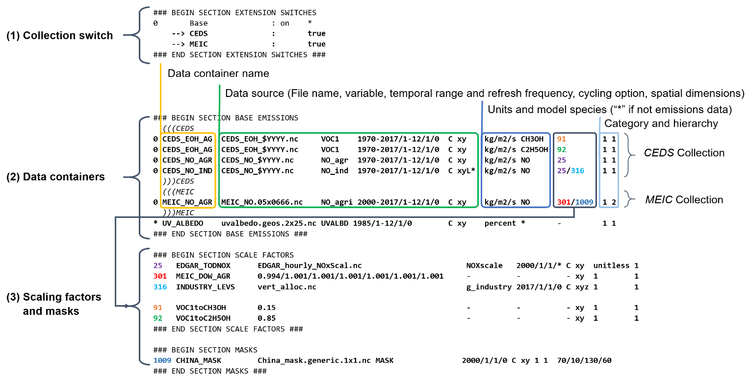
An overview of the structure and key formats of the HEMCO configuration file can be found in Figure 2 of Lin et al. [2021]:

Settings

Parameters and variables used by HEMCO are defined in between these comment lines:

###############################################################################
### BEGIN SECTION SETTINGS
###############################################################################

ROOT:                        /path/to/hemco/data/dir
METDIR:                      /path/to/hemco/met/dir
GCAPSCENARIO:                not_used
GCAPVERTRES:                 47
Logfile:                     *
DiagnFile:                   HEMCO_Diagn.rc
DiagnPrefix:                 ./OutputDir/HEMCO_diagnostics
DiagnFreq:                   00000000 010000
Wildcard:                    *
Separator:                   /
Unit tolerance:              1
Negative values:             0
Only unitless scale factors: false
Verbose:                     false
VerboseOnCores:              root       # Accepted values: root all

### END SECTION SETTINGS ###

The order within the settings section is irrelevant. Many of the settings described below are optional, and default values will be used if not explicitly set.

DiagnFile

Specifies the configuration file for the HEMCO default diagnostics collection. This file is customarily named HEMCO_Diagn.rc. For more information, please see Default diagnostics collection section.

DiagnFreq

This setting (located in the HEMCO configuration file) specifies the output frequency of the Default collection. Allowable values are:

Value	What it does
Always	Archives diagnostics on each time step.
Annually	Sets the diagnostic period to 1 year.
Daily	Sets the diagnostic period to 1 day.
End	Sets the diagnostic period so that output will only occur at the end of the simulation.
Hourly	Sets the diagnostic period to 1 hour.
Monthly	Sets the diagnostic period to 1 month
YYYYMMDD hhmnss	Sets the diagnostic period to a 15-digit string (year-month-day hour-minute-second)

Some examples of the YYYMMDD hhmmss option are:

• 00010000 000000 will generate diagnostic output once per year.

• 00000001 000000 will generate diagnostic output once per day.

• 00000000 020000 will generate diagnostic output every 2 hours.

• etc.

DiagNoLevDim

This option must be explicity added to the HEMCO configuration file. If omitted, the default behavior will be false.

Value	What it does
true	The HEMCO_diagnostics*.nc files will be created with (time,lat,lon) dimensions. [1]
false	The HEMCO_diagnostics*.nc files will always be created with (time,lev,lat,lon) dimensions.

Notes for DiagNoLevDim

[1]

But if at least one of the diagnostic quantities has a lev dimension, then the created files will have (time,lev,lat,lon) dimensions.

DiagnPrefix

Specifies the name of the diagnostic files to be created. For example:

DiagnPrefix: ./OutputDir/HEMCO_diagnostics

will create HEMCO diagnostics files in the OutputDir/ subdirectory of the run directory, and all files will begin with the text HEMCO_diagnostics.

DiagnRefTime

This option must be explicity added to the HEMCO configuration file.

By default, the value of the time:units attribute in the HEMCO_diagnostics.*.nc files will be

hours since YYYY-MM-DD hh:mn:ss`,

where YYYY-MM-DD hh:mn:ss is the diagnostics datetime. This default value can be overridden with:

DiagnRefTime: hours since 1985-01-01 00:00:00

which will reset the time:units attribute in the HEMCO_diagnostics*.nc files accordingly.

DiagnTimeStamp

This option must be explicity added to the HEMCO configuration file. If omitted, the default behavior will be End.

Value	What it does
Start	Uses the date and time at the start of the diagnostics period to timestamp diagnostic files. With this option, a 1-hour simulation from 20220101 000000 to 20220101 010000 will create a diagnostic file named HEMCO_Diagnostics.202201010000.nc.
Mid	Uses the date and time at the midpoint of the diagnostics period to o timestamp diagnostic files. With this option, a 1-hour simulation from 20220101 000000 to 20220101 010000 will create a diagnostic file named HEMCO_Diagnostics.202201010030.nc.
End	Uses the date and time at the end of the diagnostics period to timestamp diagnostic files. With this option, a 1-hour simulation from 20220101 000000 to 20220101 010000 will create a diagnostic file named HEMCO_Diagnostics.202201010100.nc.

Emission day

If present, this emission day will be used regardless of the model simulation day. If omitted, the emission day will be set to the model simulation day.

Emission hour

If present, this emission month will be used regardless of the model simulation hour. If omitted, the emisison month will be set to the model simulation hour.

Emission year

If present, this emission year will be used regardless of the model simulation year. If omitted, the emission year will be set to the model simulation year.

Emission month

If present, this emission month will be used regardless of the model simulation month. If omitted, the emission month will be set to the model simulation month.

EmisScale_<species-name>

Optional argument to define a uniform scale factor that will be applied across all inventories, categories, hierarchies, and extensions. Examples:

Value	What it does
EmisScale_NO: 1.5	Scales all NO emissions up by 50%.
EmisScale_CO: 2.0	Scales all CO emissions up by 100%.

GCAPSCENARIO

Specifies the future scenario when using GCAP meteorology. Default value: not used

GCAPVERTRES

Specifies the number of vertical levels for GCAP meteorology. Default value: 47

GridFile

Path and name of the HEMCO standalone grid description file. This is usually named HEMCO_sa_Grid.rc.

LogFile

Path and name of the output log file.

Value	What it does
*	HEMCO will write to stdout (screen output)
A file path (e.g. ./HEMCO.log)	HEMCO will open and write to that file

Note

If you are using HEMCO within CESM, then LogFile will be ignored and HEMCO will write to the CAM log file atm.log.

Mask fractions

Value	What it does
true	Fractional mask values are taken into account. This means that mask values can take any value between 0.0 and 1.0.
false	Masks are binary, and grid boxes are 100% inside or outside of a mask region. (Default setting)

METDIR

Root folder of meteorology data files that are needed for HEMCO extensions. Usually this is a subdirectory of ROOT.

MODEL

If present, the $MODEL token will be set to the value specified. If omitted, this value is determined from compiler switches.

Negative values

Value	What it does
0	No negative values are allowed (Default setting)
1	All negative values are set to zero and a warning message is printed.
2	Negative values are kept as they are.

PBL dry deposition

Value	What it does
true	Assumes that dry deposition occurs over the entire planetary boundary layer (PBL). In this case, extensions that include loss terms (e.g. air-sea exchange) will calculate a loss term for every grid box that is partly within the PBL.
false	A loss term is calculated for the surface layer only. (Default setting)

RES

If present, the $RES token will be set to the value specified. If omitted, this value is determined from compiler switches.

ROOT

Root folder containing emissions inventories and other data to be read by HEMCO.

Separator

Separator symbol. On Linux/MacOS systems, this should be set to /.

SpecFile

Path and name of the HEMCO standalone species description file. This is usually named HEMCO_sa_Spec.rc.

TimeFile

Path and name of the HEMCO standalone time description file. This is usually named HEMCO_sa_Time.rc.

Unit tolerance

Integer value denoting the tolerance against differences between the units set in the HEMCO configuration file and the netCDF units attribute found in the source file.

Value	What it does
0	No tolerance. A units mismatch will halt a HEMCO simulation.
1	Medium tolerance. A units mismatch will print a warning message, but will not halt a HEMCO simulation. (Default setting)
2	High tolerance. A units mismatch will be ignored.

Verbose

Value	What it does
true	Activates additional printout for debugging purposes.
false	Deactivates additional printout. (Default setting)

VerboseOnCores

Value	What it does
root	Restricts Verbose output to the root core. This facilitates running HEMCO in Earth System Models, where the additional overhead of printing verbose output on every core could negatively impact performance. (Default setting)
all	Prints Verbose output on all computational cores.

Wildcard

Wildcard character. On Linux/MacOS this should be set to *.

User-defined tokens

Users can specify any additional token in the Settings section section. The token name/value pair must be separated by the colon (:) sign. For example, adding the following line to the settings section would register token $ENS (and assign value 3 to it):

ENS: 3

User-defined tokens can be used the same way as the built-in tokens ($ROOT, $RES, YYYY, etc.). See sourceFile in the Base emissions for more details about tokens.

Important

User-defined token names must not contain numbers or special characters such as ., _, -, or x.

Extension switches

HEMCO performs automatic emission calculations using all fields that belong to the base emisisons extension. Additional emissions that depend on environmental parameter such as wind speed or air temperature–and/or that use non-linear parameterizations–are calculated through HEMCO extensions. A list of currently implemented extensions in HEMCO is given in Keller et al. (2014). To add new extensions to HEMCO, modifications of the source code are required, as described further in HEMCO under the hood.

The first section of the configuration file lists all available extensions and whether they shall be used or not. For each extension, the following attributes need to be specified:

ExtNr

Extension number associated with this field. All base emissions should have extension number zero. The extension number` of the data listed in section HEMCO extensions data must match with the corresponding extension number.

The extension number can be set to the wildcard character. In that case, the field is read by HEMCO (if the assigned species name matches any of the HEMCO species, see Species) but not used for emission calculation. This is particularly useful if HEMCO is only used for data I/O but not for emission calculation.

ExtName

Name of the HEMCO extension.

On/Off

Value	What it does
on	The extension will be used.
off	The extension will not be used.

Species

List of species to be used by this extension. Multiple species are separated by the Separator symbol (e.g. /). All listed species must be supported by the given extension.

• For example, the SoilNOx emissions extension only supports one species (NO). An error will be raised if additional species are listed.

Additional extension-specific settings can also be specified in the ‘Extensions Settings’ section (see also an example in Basic examples and the definition of Data collections. These settings must immediately follow the extension definition.

HEMCO expects an extension with extension number zero, denoted the Base Emisisons extension extension. All emission fields linked to the base extension will be used for automatic emission calculation. Fields assigned to any other extension number will not be inlcuded in the base emissions calculation, but they are still read/regridded by HEMCO (and can be made available readily anywhere in the model code). These data are only read if the corresponding extension is enabled.

All species to be used by HEMCO must be listed in column Species of the base extension switch. In particular, all species used by any of the other extensions must also be listed as base species, otherwise they will not be recognized. It is possible (and recommended) to use the Wildcard character, in which case HEMCO automatically determines what species to use by matching the atmospheric model species names with the species names assigned to the base emission fields and/or any emission extension.

The environmental fields (wind speed, temperature, etc.) required by the extensions are either passed from the atmospheric model or read through the HEMCO configuration file, as described in HEMCO extensions.

Base emissions

The BASE EMISSIONS section lists all base emission fields and how they are linked to scale factors. Base emissions settings must be included between these comment lines:

###############################################################################
### BEGIN SECTION BASE EMISSIONS
###############################################################################
settings go here

### END SECTION BASE EMISSIONS ###

The ExtNr field is defined in Extension switches. Other attributes that need to be defined for each base emissions entry are:

Name

Descriptive field identification name. Two consecutive underscore characters (__) can be used to attach a ‘tag’ to a name. This is only of relevance if multiple base emission fields share the same species, category, hierarchy, and scale factors. In this case, emission calculation can be optimized by assigning field names that onlydiffer by its tag to those fields (e.g. DATA__SECTOR1, DATA__SECTOR2, etc.).

For fields assigned to extensions other than the base extension (ExtNr = 0), the field names are prescribed and must not be modified because the data is identified by these extensions by name.

sourceFile

Specifies the path and name of the input file. You may include the following name tokens, which will be evaluated at runtime.

Value	What it does
$CFDIR	Refers to the location of The HEMCO configuration file.
$DD	Refers to the current simulation day (1-31).
$HH	Refers to the current simulation hour (0-23).
$MODEL	Refers to the meteorological model.
$MM	Refers to the current simulation month (1-12).
$MN	Refers to the current simulation minutes (0-59).
$RES	Refers to the model resolution.
$ROOT	Use the root directory specified in the Settings section.
$YYYY	Refers to the current simulation year.
$WD	Refers to the current day of the week (1=Sun, 2=Mon .. -7=Sat).

As an alternative to an input file, geospatial uniform values can directly be specified in the configuration file (see e.g. scale factor SO2toSO4 in Basic examples).

If multiple values are provided (separated by the separator character character), they are interpreted as different time slices. In this case, the sourceTime attribute can be used to specify the times associated with the individual slices.

If no time attribute is set, HEMCO attempts to determine the time slices from the number of data values:

# of values	Interpretation by HEMCO
7	Days of week (Sun, Mon .. Sat)
12	Months (Jan, Feb, .. Dec)
24	Hours of day (01, 02, .. 23)

Uniform values can be combined with mathematical expressions. For example, to model a sine-wave emission source, enter

MATH:2.0+sin(HH/12*PI)

Country-specific data can be provided through an ASCII file (.txt). In an ESMF environment you must specify the absolute file path rather than use the $ROOT specifier. More details on the country-specific data option are given in the Input File Format section.

If this entry is left empty (-), the filename from the preceding entry is taken, and the next 5 attributes will be ignored (see entry MACCITY_SO4 in Basic examples.

sourceVar

Source file variable of interest. Leave empty (-) if values are directly set through the sourceFile attribute or if sourceFile is empty.

sourceTime

This attribute defines the time slices to be used and the data refresh frequency. The format is year/month/day/hour. Accepted are discrete dates for time-independent data (e.g. 2000/1/1/0) and time ranges for temporally changing fields (e.g. 1980-2007/1-12/1-31/0-23). Data will automatically become updated as soon as the simulation date enters a new time interval.

The provided time attribute determines the data refresh frequency. It does not need to correspond to the datetimes of the input file.

Examples:

• If the input file contains daily data of year 2005 and the time attribute is set to 2005/1/1/0, the file will be read just once (at the beginning of the simulation) and the data of Jan 1, 2005 is used throughout the simulation.
  
  

• If the time attribute is set to 2005/1-12/1/0, the data is updated on every month, using the first day data of the given month. For instance, if the simulation starts on July 15, the data of July 1,2005 are used until August 1, at which point the data will be refreshed to values from August 1, 2005.
  
  

• A time attribute of 2005/1-12/1-31/0 will make sure that the input data are refreshed daily to the current day’s data.
  
  

• Finally, if the time attribute is set to 2005/1-12/1-31/0-23, the data file is read every simulation hour, but the same daily data is used throughout the day (since there are no hourly data in the file). Providing too high update frequencies is not recommended unless the data interpolation option is enabled (see below).

If the provided time attributes do not match a datetime of the input file, the most likely time slice is selected. The most likely time slice is determined based on the specified source time attribute, the datetimes available in the input file, and the current simulation date. In most cases, this is just the closest available time slice that lies in the past.

• For example, if a file contains annual data from 2005 to 2010 and the source time attribute is set to 2005-2010/1-12/1/0, the data of 2005 is used for all simulation months in 2005.
  
  

• More complex datetime selections occur for files with discontinuous time slices, e.g. a file with monthly data for year 2005, 2010, 2020, and 2050. In this case, if the time attribute is set to 2005-2020/1-12/1/0, the monthly values of 2005 are (re-)used for all years between 2005 and 2010, the monthly values of 2010 are used for simulation years 2010 - 2020, etc.

It is possible to use tokens $YYYY, $MM, $DD, and $HH, which will automatically be replaced by the current simulation date. Weekly data (e.g. data changing by the day of the week) can be indicated by setting the day attribute to WD (the wildcard character will work, too, but is not recommended). Weekly data needs to consist of at least seven time slices - in increments of one day - representing data for every weekday starting on Sunday. It is possible to store multiple weekly data, e.g. for every month of a year: 2000/1-12/WD/0. These data must contain time slices for the first seven days of every month, with the first day per month representing Sunday data, then followed by Monday, etc. (irrespective of the real weekdays of the given month). If the wildcard character is used for the days, the data will be interpreted if (and only if) there are exactly seven time slices. See the Input File Format section for more details. Default behavior is to interpret weekly data as ‘local time’, i.e. token WD assumes that the provided values are in local time. It is possible to use weekly data referenced to UTC time using token UTCWD.

Similar to the weekday option, there is an option to indicate hourly data that represents local time: LH. If using this flag, all hourly data of a given time interval (day, month, year) are read into memory and the local hour is picked at every location. A downside of this is that all hourly time slices in memory are updated based on UTC time. For instance, if a file holds local hourly data for every day of the year, the source time attribute can be set to 2011/1-12/1-31/LH. On every new day (according to UTC time), this will read all 24 hourly time slices of that UTC day and use those hourly data for the next 24 hours. For the US, for instance, this results in the wrong daily data being used for the last 6-9 hours of the day (when UTC time is one day ahead of local US time).

There is a difference between source time attributes 2005-2008/$MM/1/0 and 2005-2008/1-12/1/0. In the first case, the file will be updated annually, while the update frequency is monthly in the second case. The token $MM simply indicates that the current simulation month shall be used whenever the file is updated, but it doesn’t imply a refresh interval. Thus, if the source time attribute is set to $YYYY/$MM/$DD/$HH, the file will be read only once and the data of the simulation start date is taken (and used throughout the simulation). For uniform values directly set in the configuration file, all time attributes but one must be fixed, e.g. valid entries are 1990-2007/1/1/0 or 2000/1-12/1/1, but not 1990-2007/1-12/1/1.

Note

All data read from netCDF file are assumed to be in UTC time, except for weekday data that are always assumed to be in local time. Data read from the configuration file and/or from ASCII are always assumed to be in local time.

It is legal to keep different time slices in different files, e.g. monthly data of multiple years can be stored in files file_200501.nc, file_200502.nc, …, file_200712.nc. By setting the source file attribute to file_$YYYY$MM.nc and the source time attribute to 2005-2007/1-12/1/0, data of file_200501.nc is used for simulation dates of January 2005 (or any January of a previous year), etc. The individual files can also contain only a subset of the provided data range, e.g. all monthly files of a year can be stored in one file: file_2005.nc, file_2006.nc, file_2007.nc. In this case, the source file name should be set to file_$YYYY, but the source time attribute should still be 2005-2007/1-12/1/0 to indicate that the field shall be updated monthly.

This attribute can be set to the wildcard character (*), which will force the file to be updated on every HEMCO time step.

File reference time can be shifted by a fixed amount by adding an optional fifth element to the time stamp attribute. For instance, consider the case where 3-hourly averages are provided in individual files with centered time stamps, e.g.: file.yyyymmdd_0130z.nc, file.yyyymmdd_0430z.nc, …, file.yyymmdd_2230z.nc. To read these files at the beginning of their time intervals, the time stamp can be shifted by 90 minutes: 2000-2016/1-12/1-31/0-23/+90minutes. At time 00z, HEMCO will then read file 0130z and keep using this file until 03z, when it switches to file 0430z. Similarly, it is possible to shift the file reference time by any number of years, months, days, or hours. Time shifts can be forward or backward in time (use - sign to shift backwards).

CRE

Controls the time slice selection if the simulation date is outside the range provided in attribute source time (see above). The following options are available:

C

Cycling: Data are interpreted as climatology and recycled once the end of the last time slice is reached. For instance, if the input data contains monthly data of year 2000, and the source time attribute is set to 2000/1-12/1/0 C, the same monthly data will be re-used every year.

If the input data spans multiple years (e.g. monthly data from 2000-2003), the closest available year will be used outside of the available range (e.g. the monthly data of 2003 is used for all simulation years after 2003).

CS

Cycling, Skip: Data are interpreted as climatology and recycled once the end of the last time slice is reached. Data that aren’t found are skipped. This is useful when certain fields aren’t found in a restart file and, in that case, those fields will be initialized to default values.

CY

Cycling, Use Simulation Year:, Same as C, except it does not allow Emission year setting to override the simulation year.

CYS

Cycling, Use Simulation Year, Skip: Same as CS, except it does not allow Emission year setting to override the simulation year.

R

Range: Data are only considered as long as the simulation time is within the time range specified in attribute sourceTime. The provided range does not necessarily need to match the time stamps of the input file. If it is outside of the range of the netCDF time stamps, the closest available date will be used.

For instance, if a file contains data for years 2003 to 2010 and the provided range is set to 2006-2010/1/1/0 R, the file will only be considered between simulation years 2006-2010. For simulation years 2006 through 2009, the corresponding field on the file is used. For all years beyond 2009, data of year 2010 is used. If the simulation date is outside the provided time range, the data is ignored but HEMCO does not return an error—the field is simply treated as empty (a corresponding warning is issued in the HEMCO log file).

• Example: if the source time attribute is set to 2000-2002/1-12/1/0 R, the data will be used for simulation years 2000 to 2002 and ignored for all other years.

RA

Range, Averaging Otherwise: Combination of flags R and A. As long as the simulation year is within the specified year range, HEMCO will use just the data from that particular year. As soon as the simulation year is outside the specified year range, HEMCO will use the data averaged over the specified years. Here are some examples:

Setting	What this does
2015-2020/1-12/1/0 R	Uses monthly mean data only within simulation simulation years 2015-2020, and ignores the data outside of this time range.
2015-2020/1-12/1/0 A	HEMCO will always use the 2015-2020 averaged monthly values, even for simulation years 2015 through 2020.
2015-2020/1-12/1/0 RA	Uses the monthly data of the current year if the simulation year is within the range 2015-2020, and the 2015-2020 average for years before 2015 and after 2020, respectively.

RF

Range, Forced: Same as R, but HEMCO stops with an error if the simulation date is outside the provided range.

RY

Range, Use Simulation Year: Same as R, except it does not allow Emission year to override the simulation year.

RFY

Range, Forced, Use Simulation Year. Same as RY, except it does not allow Emission year to override the simulation year.

RFY3

Ranged, Forced, Use Simulation Year, 3-hourly data: Same as RFY, but used with data that is read from disk every 3 hours (e.g. meteorological data and related quantities).

E

Exact: Fields are only used if the time stamp on the field exactly matches the current simulation datetime. In all other cases, data is ignored but HEMCO does not return an error.

Example:

• sourceTime and CRE: 2013-2023/1-12/1-31/0 E

  Every time the simulation enters a new day, HEMCO will attempt to find a data field for the current simulation date. If no such field can be found in the file, the data is ignored (and a warning is prompted). This setting is particularly useful for data that is highly sensitive to date and time, e.g. restart variables.

EF

Exact, Forced: Same as E, but HEMCO stops with an error if no data field can be found for the current simulation date and time.

EC

Exact, Read/Query Contiuously..

ECF

Exact, Read/Query Continuously, Forced.

EFYO

Exact, Forced, Simulation Year, Once: Same as EF, with the following additions:

• Y: HEMCO will stop thie simulation if the simulation

  year does not match the year in the file timestamp.

• O: HEMCO will only read the file once.

This setting is typically only used for model restart files (such as GEOS-Chem Classic restart files). This ensures that the simulation will stop unless the restart file timestamp matches the simulation start date and time.

Attention

Consider changing the time cycle flag from EFYO to CYS if you would like your simulation to read a data file (such as a simulation restart file) whose file timestamp differs from the simulaton start date and time.

EY

Exact, Use Smulation Year: Same as E, except it does not allow Emission year setting to override the simulation year.

A

Averaging: Tells HEMCO to average the data over the specified range of years.

• For instance, setting sourceTime to 1990-2010/1-12/1/0 A will cause HEMCO to calculate monthly means between 1990 to 2010 and use these regardless of the current simulation date.

The data from the different years can be spread out over multiple files. For example, it is legal to use the averaging flag in combination with files that use year tokens such as file_$YYYY.nc.

I

Interpolation: Data fields are interpolated in time. As an example, let’s assume a file contains annual data for years 2005, 2010, 2020, and 2050. If sourceTime is set to 2005-2050/1/1/0 I, data becomes interpolated between the two closest years every time we enter a new simulation year. If the simulation starts on January 2004, he value of 2005 is used for years 2004 and 2005. At the beginning of 2006, the used data is calculated as a weighted mean for the 2005 and 2010 data, with 0.8 weight given to 2005 and 0.2 weight given to 2010 values. Once the simulation year changes to 2007, the weights hange to 0.6 for 2005 and 0.4 for 2010, etc. The interpolation frequency is determined by sourceTime the source time attribute.

For example, setting the source time attribute to 2005-2050/1-12/1/0 I would result in a recalculation of the weights on every new simulation month. Interpolation works in a very similar manner for discontinuous monthly,daily, and hourly data. For instance if a file contains monthly data of 2005, 2010, 2020, and 2050 and the source time attribute is set to 2005-2050/1-12/1/0 I, the field is recalculated every month using the two bracketing fields of the given month: July 2007 values are calculated from July 2005 and July 2010 data (with weights of 0.6 and 0.4, respectively), etc.

Data interpolation also works between multiple files. For instance, if monthly data are stored in files file_200501.nc, file_200502.nc, etc., a combination of source file name file_$YYYY$MM.nc and sourceTime attribute 2005-2007/1-12/1-31/0 :literal:I will result in daily data interpolation between the two bracketing files, e.g. if the simulation day is July 15, 2005, the fields current values are calculated from files file_200507.nc and file_200508.nc, respectively.

Data interpolation across multiple files also works if there are file ‘gaps’, for example if there is a file only every three hours: file_20120101_0000.nc, file_20120101_0300.nc, etc. Hourly data interpolation between those files can be achieved by setting source file to :file:file_$YYYY$MM$DD_$HH00.nc`, and sourceTime to 2000-2015/1-12/1-31/0-23 I (or whatever the covered year range is).

SrcDim

Specifies the spatial dimension of the input data and/or the model levels into which emissions will be placed. Here are some examples that illustrate its use.

SrcDim setting	What this does
xy	Specifies 2-dimensional input data
xyz	Specifies 3-dimensional input data
xy5	Emits the lowest 5 levels of the input data into HEMCO levels 1 through 5.
xy-5	Emits the tompmost 5 levels of the input data into HEMCO levels 1 through 5 (i.e. in reversed order, so that the topmost level is placed into HEMCO level 1, etc.)
xyL=5	Emits a 2-D input data field into HEMCO level 5.
xyL=2000m	Emits a 2-D input data field into the model level corresponding to 2000m above the surface.
xyL=2:5000m	Emits between HEMCO level 2 and 5000m
xyL=1:PBL	Emits from the surface (HEMCO level 1) up to the HEMCO level containing the PBL top.
xyL=PBL:5500m	Emits from the PBL top level up to 5500m.
xyL*	Emit same value to all emission levels. A scale scale factor should be applied to distribute the emissions vertically.
xyL=1:scal300	Emit from the surface (HEMCO level 1) to the injection height that is listed under scale factor 300. This scale factor may be read from a netCDF file.
xyz+"ensemble=3"	Read a netCDF file containing ensemble data (xyz plus an additional dimension named ensemble), using the 3rd ensemble member.
xyz+"ensemble=$EN"	Similar to the previous example, but using a token to denote which ensemble member to use. [2]

Notes for SrcDim

[2]

Arbitrary additional dimensions are currently not supported in a high-performance environment that uses the ESMF/MAPL input/output libraries.

SrcUnit

Units of the data.

Species

HEMCO emission species name. Emissions will be added to this species. All HEMCO emission species are defined at the beginning of the simulation (see the Interfaces section) If the species name does not match any of the HEMCO species, the field is ignored altogether.

The species name can be set to the wildcard character, in which case the field is always read by HEMCO but no species is assigned to it. This can be useful for extensions that import some (species-independent) fields by name.

ScalIDs

Identification numbers of all scale factors and masks that shall be applied to this base emission field. Multiple entries must be separated by the separator character. ScalIDs must csorrespond to the numbers provided in the Scale factors and

Note

This option only takes effect for fields that are assigned to the base extension (ExtNr = 0).

Cat

Emission category. Used to distinguish different, independent emission sources. Emissions of different categories are always added to each other.

Up to three emission categories can be assigned to each entry (separated by the separator character). Emissions are always entirely written into the first listed category, while emissions of zero are used for any other assigned category.

In practice, the only time when more than one emissions category needs to be specified is when an inventory does not separate between anthropogenic, biofuels, and/or trash emissions

For example, the CEDS inventory uses categories 1/2/12 because CEDS lumps both biofuel emissions and trash emissions with anthropogenic Because. The 1/2/12 category designation means “Put everything into the first listed category (1=anthropogenic), and set the other listed categories (2=biofuels, 12=trash) to zero.

Note

This option only takes effect for fields that are assigned to the base extension (ExtNr = 0).

Hier

Emission hierarchy. Used to prioritize emission fields within the same emission category. Emissions of higher hierarchy overwrite lower hierarchy data. Fields are only considered within their defined domain, i.e. regional inventories are only considered within their mask boundaries.

Note

This option only takes effect for fields that are assigned to the base extension (ExtNr = 0).

Scale factors

The SCALE FACTORS section of the configuration file lists all scale factors applied to the base emission field. Scale factors that are not used by any of the base emission fields are ignored. Scale factors can represent:

1. Temporal emission variations including diurnal, seasonal, or interannual variability;

2. Regional masks that restrict the applicability of the base inventory to a given region; or

3. Species-specific scale factors, e.g., to split lumped organic compound emissions into individual species.

This sample snippet of the HEMCO configuration file shows how scale factors can either be read from a netCDF file or listed as a set of values.

###############################################################################
### BEGIN SECTION SCALE FACTORS
###############################################################################
# ScalID Name srcFile srcVar srcTime CRE Dim Unit Oper

# %%% Hourly factors, read from disk %%%
1 HOURLY_SCALFACT hourly.nc                                      factor 2000/1/1/0-23 C xy 1 1

# %%% Scaling SO2 to SO4 (molar ratio) %%%
2 SO2toSO4        0.031                                          -      -             - -  1 1

# %%% Daily scale factors, list 7 entries %%%
20 GEIA_DOW_NOX   0.784/1.0706/1.0706/1.0706/1.0706/1.0706/0.863 -      -             - xy 1 1

### END SECTION SCALE FACTORS ###

Options sourceFile, sourceVar, sourceTime, CRE, SrcDim, and SrcUnit are described in Base emissions.

Scale factor options not previously described are:

ScalID

Scale factor identification number. Used to link the scale factors to the base emissions through the corresponding ScalIDs attribute in Base emissions.

Oper

Scale factor operator. Determines the operation performed on the scale factor. Possible values are:

Oper	What this does
1	Multiplication (Emission = Base * Scale)
-1	Division (Emission = Base / Scale)
2	Squared (Emission = Base * Scale**2)

MaskID

Optional. ScalID of a mask field. This optional value can be used if a scale factor shall only be used over a given region. The provided MaskID must have a corresponding entry in the Masks section of the configuration file.

Note

Scale factors are assumed to be unitless (aka 1) and no automatic unit conversion is performed.

Masks

This section lists all masks used by HEMCO. Masks are binary scale factors (1 inside the mask region, 0 outside). If masks are regridded, the remapped mask values (1 and 0) are determined through regular rounding, i.e. a remapped mask value of 0.49 will be set to 0 while 0.5 will be set to 1.

The MASKS section in the HEMCO configuration file will look similar to this (it will vary depending on the type of GEOS-Chem simulation you are using):

 ###############################################################################
 ### BEGIN SECTION MASKS
 ###############################################################################
 # ScalID Name sourceFile sourceVar sourceTime CRE SrcDim SrcUnit Oper Lon1/Lat1/Lon2/Lat2

 #==============================================================================
 # Country/region masks
 #==============================================================================
 1000 EMEP_MASK   EMEP_mask.geos.1x1.20151222.nc           MASK     2000/1/1/0 C xy unitless 1 -30/30/45/70
 1002 CANADA_MASK Canada_mask.geos.1x1.nc                  MASK     2000/1/1/0 C xy unitless 1 -141/40/-52/85
 1003 SEASIA_MASK SE_Asia_mask.generic.1x1.nc              MASK     2000/1/1/0 C xy unitless 1  60/-12/153/55
 1004 NA_MASK     NA_mask.geos.1x1.nc                      MASK     2000/1/1/0 C xy unitless 1 -165/10/-40/90
 1005 USA_MASK    usa.mask.nei2005.geos.1x1.nc             MASK     2000/1/1/0 C xy unitless 1 -165/10/-40/90
 1006 ASIA_MASK   MIX_Asia_mask.generic.025x025.nc         MASK     2000/1/1/0 C xy unitless 1 46/-12/180/82
 1007 NEI11_MASK  USA_LANDMASK_NEI2011_0.1x0.1.20160921.nc LANDMASK 2000/1/1/0 C xy 1        1 -140/20/-50/60
 1008 USA_BOX     -129/25/-63/49                           -        2000/1/1/0 C xy 1        1 -129/25/-63/49

### END SECTION MASKS ###

The required attributes for mask fields are described below:

Options ScalID and Oper are described in Scale factors.

Options sourceFile, sourceVar, sourceTime, CRE, SrcDim, and SrcUnit are described in Base emissions.

The Box option is deprecated.

Instead of specifying the sourceFile and sourceVar fields, you can directly provide the lower left and upper right box coordinates: Lon1/Lat1/Lon2/Lat2 . Longitudes must be in degrees east, latitudes in degrees north. Only grid boxes whose mid points are within the specified mask boundaries. You may also specify a single grid point (Lon1/Lat1/Lon1/Lat1/).

Caveat for simulations using cropped horizontal grids

Consider the following combination of global and regional emissions inventories:

In the Base Emissions section:

0 GLOBAL_INV_SPC1   ...  SPC1 -     1 5
0 INVENTORY_1_SPC1  ...  SPC1 1001  1 56
0 INVENTORY_2_SPC1  ...  SPC1 1002  1 55

In the Masks section:

1001 REGION_1_MASK ... 1 1 70/10/140/60
1002 REGION_2_MASK ... 1 1 46/-12/180/82

For clarity, we have omitted the various elements in these entries of HEMCO_Config.rc that are irrelevant to this issue.

With this setup, we should expect the following behavior:

1. Species SPC1 should be emitted globally from inventory GLOBAL_INV (hierarchy = 5).
   
   

2. Regional emissions of SPC1 from INVENTORY_1 (hierarchy = 56) should overwrite global emissions in the region specified by REGION_1_MASK.
   
   

3. Likewise, regional emissions of SPC1 from INVENTORY_2 (hierarchy = 55) should overwrite global emissions in the region specified by REGION_2_MASK.
   
   

4. In the locations where REGION_2_MASK intersects REGION_1_MASK, emissions from INVENTORY_1 will be applied. This is because INVENTORY_1 has a higher hierarchy (56) than INVENTORY_2 (55).

When running simulations that use cropped grids, one or both of the boundaries specified for the masks (70/10/140/60 and 46/-12/180/82) in HEMCO_Config.rc can potentially extend beyond the bounds of the simulation domain. If this should happen, HEMCO would treat the regional inventories as if they were global, the emissions for the highest hierarchy (i.e., INVENTORY_1) would be applied globally. Inventories with lower hierarchies would be ignored.

Tip

Check the HEMCO log output for messages to make sure that none of your desired emissions have been skipped.

The solution is to make the boundaries of each defined mask region at least a little bit smaller than the boundaries of the nested domain. This involves inspecting the mask itself to make sure that no relevant gridboxes will be excluded.

For example, assuming the simulation domain extends from 70E to 140E in longitude, using this mask definition:

1001 REGION_1_MASK ... 1 1 70/10/136/60

would prevent INVENTORY_1 from being mistakely treated as a global inventory. We hope to add improved error checking for this condition into a future HEMCO version.

Data collections

The fields listed in the HEMCO configuration file data collections. Collections can be enabled/disabled in section extension switches. Only fields that are part of an enabled collection will be used by HEMCO.

The beginning and end of a collection is indicated by an opening and closing bracket, respectively: (((CollectionName and )))CollectionName. These brackets must be on individual lines immediately preceeding / following the first/last entry of a collection. The same collection bracket can be used as many times as needed.

The collections are enabled/disabled in the Extension Switches section (see Extension Switches). Each collection name must be provided as an extension setting and can then be readily enabled/disabled:

###############################################################################
#### BEGIN SECTION EXTENSION SWITCHES
###############################################################################
# ExtNr ExtName           on/off  Species
0       Base              : on    *
    --> MACCITY           :       true
    --> EMEP              :       true
    --> AEIC              :       true

### END SECTION EXTENSION SWITCHES

###############################################################################
### BEGIN SECTION BASE EMISSIONS
###############################################################################
ExtNr Name srcFile srcVar srcTime CRE Dim Unit Species ScalIDs Cat Hier

(((MACCITY
0 MACCITY_CO MACCity.nc  CO 1980-2014/1-12/1/0 C xy  kg/m2/s CO 500      1 1
)))MACCITY

(((EMEP
0 EMEP_CO    EMEP.nc     CO 2000-2014/1-12/1/0 C xy  kg/m2/s CO 500/1001 1 2
)))EMEP

(((AEIC
0 AEIC_CO    AEIC.nc     CO 2005/1-12/1/0      C xyz kg/m2/s CO -        2 1
)))AEIC

### END SECTION BASE EMISSIONS ###

###############################################################################
#### BEGIN SECTION SCALE FACTORS
###############################################################################
# ScalID Name srcFile srcVar srcTime CRE Dim Unit Oper

500 HOURLY_SCALFACT $ROOT/hourly.nc factor  2000/1/1/0-23 C xy 1 1
600 SO2toSO4        0.031           -       -             - -  1 1

### END SECTION SCALE FACTORS ###

###############################################################################
#### BEGIN SECTION MASKS
###############################################################################
#ScalID Name srcFile srcVar srcTime CRE Dim Unit Oper Box

1001 MASK_EUROPE $ROOT/mask_europe.nc MASK 2000/1/1/0 C xy 1 1 -30/30/45/70

### END SECTION MASKS ###

Extension names

The collection brackets also work with extension names, e.g. data can be included/excluded based on extensions. This is particularly useful to include an emission inventory for standard emission calculation if (and only if) an extension is not being used (see example below).

Undefined collections

If, for a given collection, no corresponding entry is found in the extensions section, it will be ignored. Collections are also ignored if the collection is defined in an extension that is disabled. It is recommended to list all collections under the base extension.

Exclude collections

To use the opposite of a collection switch, .not. can be added in front of an existing collection name. For instance, to read file NOT_EMEP.nc only if EMEP is not being used:

(((.not.EMEP
0 NOT_EMEP_CO    $ROOT/NOT_EMEP.nc     CO 2000/1-12/1/0 C xy kg/m2/s CO 500/1001 1 2
))).not.EMEP

Combine collections

Multiple collections can be combined so that they are evaluated together. This is achieved by linking collection names with .or.. For example, to use BOND biomass burning emissions only if both GFED and FINN are not being used:

(((.not.GFED.or.FINN
0 BOND_BM_BCPI   $ROOT/BCOC_BOND/v2014-07/Bond_biomass.nc BC   2000/1-12/1/0 C xy kg/m2/s BCPI 70 2 1
0 BOND_BM_BCPO   -                                        -    -             - -  -       BCPO 71 2 1
0 BOND_BM_OCPI   $ROOT/BCOC_BOND/v2014-07/Bond_biomass.nc OC   2000/1-12/1/0 C xy kg/m2/s OCPI 72 2 1
0 BOND_BM_OCPO   -                                        -    -             - -  -       OCPO 73 2 1
0 BOND_BM_POA1   -                                        -    -             - -  -       POA1 74 2 1
))).not.GFED.or.FINN